Get free samples written by our Top-Notch subject experts for taking online Assignment Help services.
In this above it is given the details of this topic is
AADT=35000 veh/day
D=0.55
PHF=0.85
PT=5%
PB = 6%
PR = 5%
So here we wot the formula value is
DDHV= 0.12*0.55*35000
=2310 v/h
Below also it is needed to calculate the lane number and also get idea about the hourly volume as well as also get the peak hour factor are provided the below
SF= DDHV/PHF
=2310/0.85
=2717.65
So now we have to calculate the needed the road number. Equation 4.18 will be arrange as belows
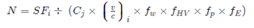
So as per this equation is the value is
CJ = 2000 “(design speed = 70mph)”
fw=1
Fhv= 1
Fp = 1
fE = 1
Putting the value of this formula is
N= 2717/(2000*0.71*1*1*1*1)
Therefore N= 1.91
Therefore it is need to three lane for every direction
“Table 4.2 Ratios of flow to capacity for different levels of service and design
Speeds (Source: Highway Capacity Manual (TRB, 1985))”
|
Level of service |
v/c C70 |
v/c C60 |
v/c C50 |
|
A |
0.37 |
0.31 |
|
|
B |
0.55 |
0.51 |
0.55 |
|
C |
0.72 |
0.62 |
0.7 |
|
D |
0.82 |
0.79 |
0.75 |
|
E |
1 |
1 |
1 |
|
F |
Variable |
Variable |
Variable |
1.2
Prove the better solution between this and a) increasing the area to impediment from traveled edge to 1.22 m, or b) reordering the entire route over more than a types of road from "mountainous" to "rolling." here it is discussing as well as justify this same results obtained in a critical manner (Avramenko. and Zyhun, 2021).
Here DDHV = design of hourly volume * Direction of movement factor
Here provide the peak hour factor is will be define as like the ratio of the hourly volume to a in excess of 15 min flow rate to expended to a hourly volume
SF= DDHV/PHF
=2310/0.85
=2717.65
So now we have to calculate the needed the road number. Equation 4.18 will be arrange as below
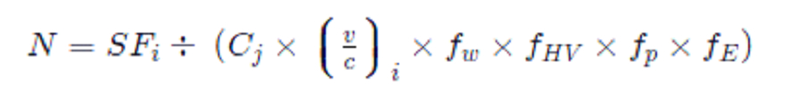
So as per this equation is the value is
CJ = 2000 “(design speed = 70mph)”
fw=1
Fhv= 1
Fp = 1
fE = 1
Putting the value of this formula is
N= 2717/(2000*0.71*1*1*1*1)
Therefore N= 1.91
Therefore it is need to three lane for every direction and here the one lane is reduction for every direction so then the vehicle transport is will reduce and also as per daily basis.
1.3
Other possible solutions (furthermore in mixture) that could decreases the amount of routes on the concerned highway (Hint: maintain the very next things constant: partitioned multi-lane agreement; AADT = 35000 vehicles per day; Design Speed = 70 miles per hour; "ideal" driver citizenry; PHF = 0.85; D = 0.55) to support your claim, give step-by-step computations. A Collectible job is to collect data. Even when both of them have been classified as Collectors, the new classification system may experience unwanted redundancy. Unless other factors are equal, the route with both the greater AADT would've been assigned the Collectors designation, whereas its counterpart would be assigned this same Local category. Moreover, when determining whichever of several (or even more) identical as well as sequence of events that incrementally roadways must be categorized with such a higher (or less) category than another, AADT is sometimes employed as just a "tie-breaker (Badassa, et al. 2020)”. Consider the situation where two parallel streets appear to operate as a Bridge. Although both of those were being classified as Collectors, the new classification system may experience unwanted redundancy. Unless other factors are equal, the route with the greater AADT would've been assigned the Collector designation, whereas its counterpart would be assigned this same Local category.
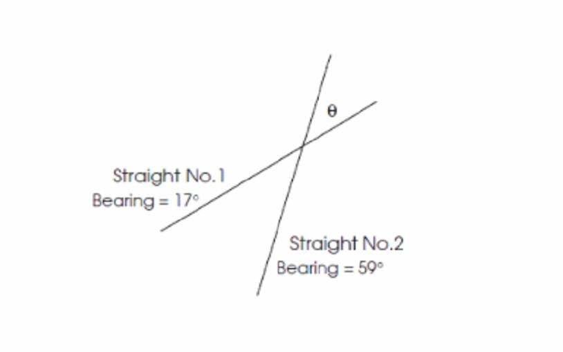
Figure 1: Plot of transit curve as x and y coordination
(Sources: chrome-extension://efaidnbmnnnibpcajpcglclefindmkaj/viewer.html)
The design speed 6.55 km/h
Therefore the desirable minimum radius is 510 m here the super elevation is taken is 7%
Length of transition
By using the equation is 6.25
L={V^{3}}/left (3.6^{3}\times C\times R\right)}
L=V3/(3.63*C*R)
Therefore L={6.55^{3}}/left (3.6^{3}\times 0.45\times 510\right)}
L=6.55 3/(3.63*0.45*510)
L= 0.03m
The equation 6.26 dictate which transition will be no greater than “(24R)^{0.5}(24R)0.5”.
In that case:
L_{max}= \sqrt{24R} = \sqrt{24×510}=110.6 m>0.03 mLmax=24R=24×510=110.6m>0.03 m
Consequently the length which is derived is lesser than the “maximum permissible value”.
Shift:
The the use of this Equation 6.24:
S={L^{2}}/{24R}
={(0.03)^{2}}÷{24×510}S
=L2/24R
=(0.03)2÷24×510
=7.35* 10^8 m
Length of IT:
By the use of this Equation 6.29:
IT=\left(R+S\right)\tan \left({\theta }/{2}\right)+{L}/{2}IT
=(R+S)tan(θ/2)+L/2
IT=\left(510.605\right)\tan \left({42}/{2}\right)+{86.03}/{2}IT
=(510.605)tan(29/2)+0.03/2
=132.05m
Form of the transition curve:
By the us of this Equation 6.31:
x=y^{3} \div 6RLx =y3÷6RL
=y^{3} \div 6×510×0.03 =y3÷6×510×0..03
=y^{3} \div 91.8 =y3÷91.8…………………………..equation 6.32
Coordinates of the place where the circular arc begins: When y matches the transitioning length, this happens (0.03 m). That's when it gets interesting.
By the use of this Equation 6.31:
x=L^{3} \div 6RL=L^{2} \div 6Rx=L3÷6RL=L2÷6R
x=(0.03)^{2} \div (6×510)x=(0.03)2÷(6×510)
=2.94 * 10^7 m
During both endpoints of something like the arc of circular, this position could now be adjusted. We can now sketch the circle because we understand its radius (Ignaccolo and Tiboni, 2021).
Note: Note that a series consecutive offsets must always be produced before the curve can be plotted. Its offset duration for intermediary y - value generally usually around 10 – 20 meters. Using this Equation 6.32 and a 10m offsetting length, then value for x anywhere at range y all along straight connecting the tangential point towards the corresponding points, using tangential point as that of the center (0,0), were which can be seen in Tables 6.10.
In the below table 6.10 the offsets at the 10 meter intervals
Line graph
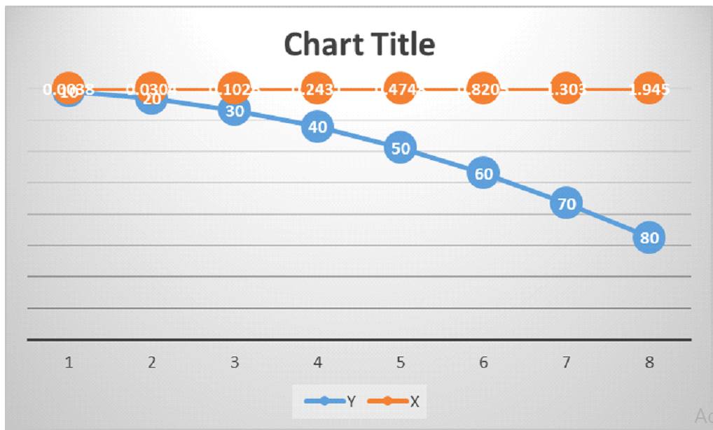
Figure 2: Line chart of X and Y
(Sources: MS-Excel)
|
Y |
X |
|
10 |
0.0038 |
|
20 |
0.0304 |
|
30 |
0.1026 |
|
40 |
0.2431 |
|
50 |
0.4748 |
|
60 |
0.8205 |
|
70 |
1.303 |
|
80 |
1.945 |
2.7
L={V^{3}}/left (3.6^{3}\times C\times R\right)}
L=V3/(3.63*C*R)
Therefore L={6.55^{3}}/left (3.6^{3}\times 0.45\times 510\right)}
L=6.55 3/(3.63*0.45*510)
L= 0.03m
2= 0.7
“(24* 510)^{0.5}(24510)0.5”.
Therefore the equation is
L_{max}= \sqrt{24R} = \sqrt{24×510}=110.6 m>0.03 mLmax=24R=24×510=110.6m>0.03 m
consequently the length which is derived is lesser than the “maximum permissible value”.
The the use of this Equation 6.24:
S={L^{2}}/{24R}
={(0.03)^{2}}÷{24×510}S
=L2/24R
=(0.03)2÷24×510
=7.35* 10^8 m
By the use of this Equation 6.29:
IT=\left(R+S\right)\tan \left({\theta }/{2}\right)+{L}/{2}IT
=(R+S)tan(θ/2)+L/2
IT=\left(510.605\right)\tan \left({42}/{2}\right)+{86.03}/{2}IT
=(510.605)tan(29/2)+0.03/2
=132.05m
By the us of this Equation 6.31:
x=y^{3} \div 6RLx =y3÷6RL
=y^{3} \div 6×510×0.03 =y3÷6×510×0..03
=y^{3} \div 91.8 =y3÷91.8…………………………..equation 6.32
Coordinates of the place where the circular arc begins: When y matches the transitioning length, this happens (0.03 m). That's when it gets interesting.
x=L^{3} \div 6RL=L^{2} \div 6Rx=L3÷6RL=L2÷6R
x=(0.03)^{2} \div (6×510)x=(0.03)2÷(6×510)
=2.94 * 10^7 m
L={V^{3}}/left (3.6^{3}\times C\times R\right)}
L=V3/(3.63*C*R)
Therefore L={6.55^{3}}/left (3.6^{3}\times 0.45\times 510\right)}
L=6.55 3/(3.63*0.45*510)
L= 0.03m
2= 0.5
L= {V^{3}}/{\left(3.6^{3} \times C \times R \right) }L=V3/(3.63×C×R)
L= {85^{3}}/{\left(3.6^{3} \times 0.3\times 510\right) }L=853/(3.63×0.3×510)
=86.03 m
(24R)^{0.5}(24R)0.5.
In that case:
L_{max}=\sqrt{24R} =\sqrt{24×510}=110.6 m>86.03 mLmax=24R=24×510=110.6m>86.03m
Therefore the derived length is less than the maximum permissible value.
Shift:
Using Equation 6.24:
S={L^{2}}/{24R}={(86.03)^{2}}÷{24×510}S=L2/24R=(86.03)2÷24×510
=0.605 m
Length of IT:
Using Equation 6.29:
IT=\left(R+S\right)\tan \left({\theta }/{2}\right)+{L}/{2}IT=(R+S)tan(θ/2)+L/2
IT=\left(510.605\right)\tan \left({42}/{2}\right)+{86.03}/{2}IT=(510.605)tan(42/2)+86.03/2
=196.00+43.015
=239.015 m
Form of the transition curve:
Using Equation 6.31:
x=y^{3} \div 6RLx=y3÷6RL
=y^{3} \div 6×510×86.03=y3÷6×510×86.03
=y^{3} \div 263 251.8=y3÷263251.8 (6.320
x=L^{3} \div 6RL=L^{2} \div 6Rx=L3÷6RL=L2÷6R
x=(86.03)^{2} \div (6×510)x=(86.03)2÷(6×510)
=2.419 m
The types of pavements were modelled as a multiple structure, with the linear viscoelastic model used to calculate stresses along with the strains at important places (Malekjafarian et al. 2018). The following 3 kinds of surface defects arising from repetitive (cyclic) transmission of traffic volumes are studied in order to evaluate the characteristics of achievement: Vertical compressional strain just at bottom of the semi, which might results in comment thread deformation and deformations somewhere at road surface.
As demonstrated in Figure 1, lowering the maximum velocity restriction besides 5 km / h out from 85th median speed could disproportionately affect 23% of something like the vehicles with in traffic flows (Nikolaeva. and Sakhapov, 2020). As a result, the 85th % speed number is regarded as such speed of traffic which most strongly matches the safe along with the reasonable velocity.
Reference List
Journals
Avramenko, Y.O. and Zyhun, A.Y., 2021. ENGINEERING STRUCTURES OF UNDERGROUND TRANSPORT INFRASTRUCTURE. Publishing House “Baltija Publishing”.
Badassa, B.B., Sun, B. and Qiao, L., 2020. Sustainable transport infrastructure and economic returns: A bibliometric and visualization analysis. Sustainability, 12(5), p.2033.
Ignaccolo, M. and Tiboni, M., Transport infrastructure and systems in a changing world: towards a safer mobility.
Malekjafarian, A., OBrien, E.J. and Golpayegani, F., 2018. Indirect monitoring of critical transport infrastructure: Data analytics and signal processing. In Data analytics for smart cities (pp. 143-162). Auerbach Publications.
Nikolaeva, R. and Sakhapov, R., 2020, July. Improving transport infrastructure in the context of the transition to the smart city concept in small towns. In IOP Conference Series: Materials Science and Engineering (Vol. 890, No. 1, p. 012215). IOP Publishing.
Pluskal, J., Šomplák, R. and Kudela, J., 2021. Novel Approaches for Transport Infrastructure Reduction to Effective Optimisation of Flow Tasks. Chemical Engineering Transactions, 88, pp.463-468.
Pushkarev, A., Podoprigora, N. and Dobromirov, V., 2018. Methods of providing failure-free operation in transport infrastructure objects. Transportation Research Procedia, 36, pp.634-639.
Svalova, A., Helm, P., Prangle, D., Rouainia, M., Glendinning, S. and Wilkinson, D.J., 2021. Emulating computer experiments of transport infrastructure slope stability using Gaussian processes and Bayesian inference. Data-Centric Engineering, 2.
Tudorica, A., Banacu, C.S. and Colesca, S.E., 2021. A LITERATURE REVIEW REGARDING THE APPLICATION OF MULTI-CRITERIA ANALYSIS IN TRANSPORT INFRASTRUCTURE PROJECTS. Management Research & Practice, 13(2).
Vlahini? Lenz, N., Pavli? Skender, H. and Mirkovi?, P.A., 2018. The macroeconomic effects of transport infrastructure on economic growth: the case of Central and Eastern EU member states. Economic research-Ekonomska istra�ivanja, 31(1), pp.1953-1964.
Yucelgazi, F. and Yitmen, I., 2019, February. Risk Assessment for Large-Scale Transport Infrastructure Projects. In IOP Conference Series: Materials Science and Engineering (Vol. 471, No. 2, p. 022005). IOP Publishing.
Zegras, C., Transport infrastructure and systems in a changing world: towards sustainable mobility planning.
Get Better Grades In Every Subject
Submit Your Assignments On Time
Trust Academic Experts Based in UK
Your Privacy is Our Topmost Concern
offer valid for limited time only*