BU7045 Quantitative Techniques for Financial Analysis Assignment Sample

• Type Assignment
• Downloads558
• Pages13
• Words3200

Introduction

Quantitative Techniques for Financial Analysis are an appropriate and effective method that helps and supports mathematical and statistical analysis of an organization’s financial health properly. Most importantly it mostly allows for the analysis of big datasets, allowing them to make informed investment judgments by recognizing ways, anticipating market movements, evaluating risks, and optimizing portfolios founded on objectives. Also, it effectively delivers a data-driven approach to financial decision-making. Students who face challenges in applying these techniques can benefit from help with assignment writing to ensure clarity and accuracy in their analyses. Most importantly to choose four same sector-related organizations to calculate their 15-year profitability ratio, operational ratios, structure ratios, and employee ratios. The selected organizations are BP Plc, Harbour Energy Plc, Tullow Oil Plc, and Shell Plc these organizations are mostly selected for these are listed in FTSE100. Moreover, this analysis has an appropriate purpose which is to critically and statistically analyze the financial health of those chosen organisations and help organisations to make some effective decisions to incense organisational growth and sustainability. Most importantly this analysis is mostly conducted by descriptive analytics, comparing organisational performance, determinants of profitability, time series analysis, and beta analysis. The analysis also has some potential objectives which are represented below-

• To represent descriptive analysis by using any three ratios.
• To examine a significant difference between the organisational performance through t-test analysis.
• To investigate organisational profitability by using structure, operational, and employee ratios.
• To examine the immediate share price is a good predictor of current share prices of chosen organizations by using time series analysis.
• To estimate the beta for the regression coefficient between the returns of chosen companies.

Descriptive Analysis

Descriptive statistics is mostly an appropriate statistical method that helps to significantly summarize a big data set. Which can be either a model of the entire people or representative of a population. This tool is mostly broken down into steps of main tendency and estimates of variability (Chen et al. 2022). Measurements of central tendency include the median, mean, and mode, while estimates of variability contain variance, standard deviation, maximum variables, and minimum skewness and kurtosis. In this analysis, Quantitative Techniques for Financial Analysis are applied to evaluate profit margin, current ratio, and interest cover across four companies, providing a data-driven foundation for understanding organizational financial health.

Table 1: Descriptive Statistics

The above table mainly represents descriptive statistics of four different types of organization’s those are BP Plc, Harbour Energy Plc, Tullow Oil Plc, and Shell Plc financial ratios those ratios are profit margin, current ratio, and interest coverage. As per the above figure, it was easy to understand the average profit margin stands at 2.963833333, indicating that, on average, the entities in the sample are operating at a loss. The standard error is 4.24286597, suggesting moderate precision around the mean. The median profit margin is 7.275, which is substantially more positive than the mean. This disparity may indicate a skew in the data, suggesting outliers may be pulling the mean down. Also, the observed range is 145.86, with a minimum of 98.26 and a maximum of 47.6. This reflects significant variability in profit margins between entities. Moreover, the current ratio ranges from a minimum of 0.14 to a maximum of 1.72, with a total range of 1.58, demonstrating variation in liquidity among the sampled entities. Most importantly according to the descriptive statistics, the interest cover ranges from a minimum of 13.3 to a maximum of 41.56, making the observed range 54.86, which highlights significant differences in the capacity to cover interest across the entities.

However, this significant analysis mostly reveals different characteristics in the data across the three financial metrics. The profit margin is represented by negative averages and high variability, suggesting financial challenges for many of the entities (Yuan et al. 2022). The current ratio indicates a reasonable level of liquidity, while the interest cover suggests a robust capacity for meeting interest expenses. Understanding these metrics will be essential for stakeholders when assessing the overall financial health of the entities involved. Also, as per the standard deviation values, it was easy to recognize that the data set does not have many outliers that can generate an effect on the significant result (Sullivan et al. 2021). Moreover, the skewness is 1.465115691, indicating the distribution's symmetry further analysis would be needed to understand its implications. Also, the average interest cover is 6.564, which points to the strong ability of the entities to meet their interest obligations.

Comparing the Performance of the Companies

This section mainly compares the performance of the selected organisation. The compression is significantly represented through Anova testing. ANOVA is a test utilized to resolve differences between study results from three or more irrelevant samples or groups (Yu et al. 2022). Moreover, to significantly generate good quality depth to the overall composition two null and alternative hypotheses are represented below-

H0 There is no relationship between the profit margin of the companies

H1 There is a relationship between the profit margin of the companies

Table 2: ANOVA Test

BU7045 Quantitative Techniques for Financial Analysis Assignment Sample

Liked This Sample? Hire Me Now

Alan Turner 9 Years | MSc

The above figure mainly represents and evaluates the relationship between the profit margins of four different companies BP Plc, Harbour Energy PLC, Shell PLC, and Tullow Oil PLC, using ANOVA to determine if there are statistically significant differences in performance among them. As per the above figure, it was easy to understand the P-value of 17% means that there is no good evidence to reject the null hypothesis (H0) (Tsushima, 2022). This implies that there cannot be a statistically meaningful difference in the profit margins across the four companies at the conventional alpha level of 0.05. The conflict for Harbour Energy PLC is notably high at 1246.3152, demonstrating a high degree of variability in profit margins within that company. This may be due to uneven performance over the estimated period. Moreover, the F-statistic, calculated as 1.7211452, reached the F critical value of 2.7694309. Since the F-statistic does not transcend the F critical, this supports the decision to fail to reject the null hypothesis.

Most importantly as per the overall compression, it was easy to recognize BP Plc and Shell PLC offer positive moderate profit margins of 3.498 and 6.728 respectively, indicating stable profitability. However, both Harbour Energy PLC and Tullow Oil PLC display negative profit margins, suggesting challenges in maintaining profitability. Also, as per the overall analysis, it was easy to recognize that there is no significant relationship between the profit margins of BP Plc, Harbour Energy PLC, Shell PLC, and Tullow Oil PLC. However, it emphasizes variabilities within the groups, especially for Harbour Energy and Tullow Oil, showing potential areas for further investigation into operational efficiencies and market conditions affecting their performances. The businesses with positive averages (BP and Shell) may also represent more stable investment opportunities based on their current profit margins.

Time Series Analysis

Time series analysis is a statistical technique that examines data points accumulated over a period. It allows for identifying practices, movements, and behaviors in data. This approach can help institutions make advised decisions and forecasts (Diggle & Giorgi 2024). In this process, time service analysis is going to be conducted with the help of three months of daily stock price data of Shell Plc. The main reason behind the analysis was to find the relevance of the company’s current share price with its historical share price. The analysis was conducted with the help of the auto-regression method of four lag days (Lucky, & Elfreda 2024). This method of evaluating the relation of current share prices with historical share prices was relevant to the Effective Marketing Hypothesis. This particular investment theory suggests that there is a direct relation between the prices of stocks with other relevant market information (Haddad et al. 2021). The fluctuation in the shared piece in the current time is reflected in both the past and future value of the same share prices. The present timing strategy can be very useful for investors in the process of adapting to market changes and price fluctuations.

There were also other stock market predicates that can be used in this process such as fundamental analysis capital economics and moving average. However, this lagged-moving method was beneficial because of its accuracy in forecasting the prices of future securities. In the autoregression, the dependent variable was the actual share price value of the stocks, and the independent variable was the four lagged values of the stocks.

Hypothesis

H0 (Null Hypothesis): There is no significant relationship between the actual share price value of the stocks and its four lagged values.

H1 (Alternate Hypothesis): There is a significant relationship between the actual share price value of the stocks and its four lagged value

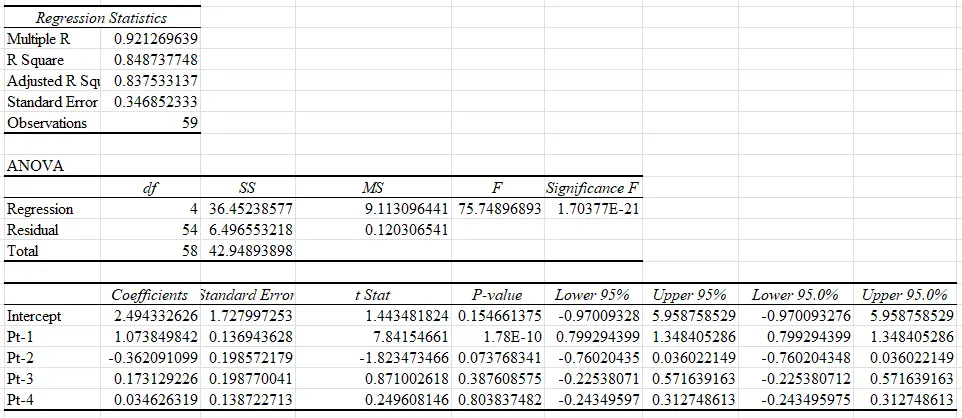
Table 3: Auto Regression

The above table shows the value result of auto-regression analysis which was conducted with the three-month share price value of Shel Plc. The four-day lag value was taken from the sales stock price data of the company. In the conducted regression analysis, both the values of R and R Square were 0.848 and 0.837. The R-value is grated that the minimal value range of 0.7 which indicates both strong and positive relation between the actual share precise and the four lagged share prices. The R-square value of the company was also high showing a good fit of the regression line with the data. The P-values of the four lagged stock prices were greater than the ideal value of 0.05 except for lag 1 which is very small. The t-state values are very high (7.841) for P(t-1) which indicates that there is a significant difference between the actual prices and the lagged price value of the stock.

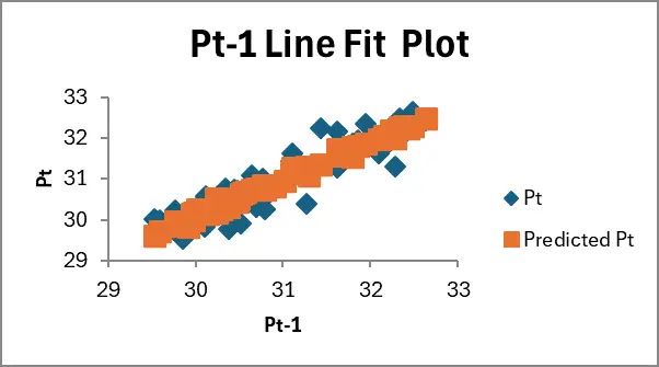
Figure 1: Lag Day 1 Line Fit Plot

The above figure mainly represents the linear fit plot of the first lag day. As per the provided figure, it was easy to understand the blue line indicates the price and the orange line indicates the predicted price. The figure states that the price points which are indicated by the blue points are spearheaded by the comparison of the predicted value of the stock price. This indicates a potential wake-positive autocorrelation between the actuarial prices of the stock and the lagged price of the stock.

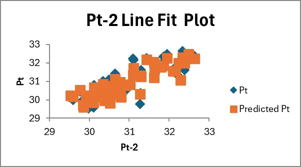
Figure 2: Lag Day 2 Line Fit Plot

As per the provided figure, it was easy to recognize there is an appropriate and powerful linear practice along the diagonal that indicates meaningful positive autocorrelation. This significant plot is mainly evaluated by time series calculation. Most importantly through this significant plot, it was easy to understand the predicted Pt is higher than the actual Pt. Because of this significant figure, it was easy to understand the data set-related samples are significantly clustered with each other which is the main reason for understanding the positive autocorrelation between predicting Pt and actual Pt.

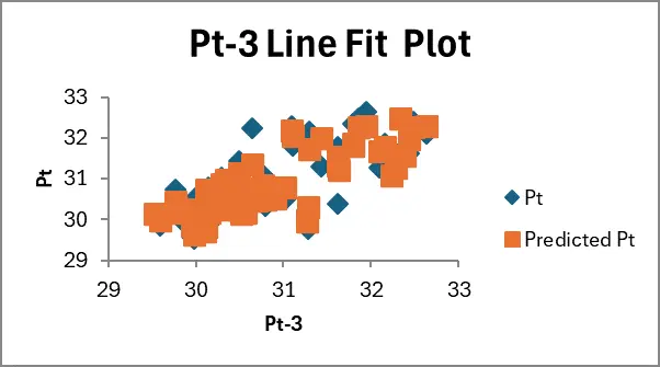
Figure 3: Lag Day 3 Line Fit Plot

The above figure shows the lune fit plot of the third lagged day value of Shel’s share price. The graph highlights that although the predicted value of the prices was on top of the lagged day price value the plots do not follow linear patterns. This particular pattern indicates a strong relation between the actuarial prices and the predicted price of the stock. The relation between the variables was non-linear.

Figure 4: Lag Day 4 Line Fit Plot

As per the above lag, 4 lines fit the plot it was easy to recognize there is a strong positive relationship between price and predicting price. Also, the predicted plots directly overlap the actual prices of the lag values showing a high correlation among them. Most importantly this is appropriate and the most potential way to understand if there is significant positive autocorrelation or weak positive autocorrelation between Pt means price and Predicted Pt (price). As per the overall analysis, it was easy to understand there is a positive correlation between these factors.

Most importantly as per the overall analysis, it was easy to conclude that for the first factor, the alternative hypothesis is accepted means “There is a significant relationship between the actual share price value of the stocks and its four lagged values”. Because the first factor’s p-value was 1.77819596887615E-10. However, for other factors, the null hypothesis is rejected because the Pt 2 factor’s p-value was 0.0737683410225177, the Pt 3 factor’s p-value was 0.871002617618819, and the Pt 4 factor’s p-value was 0.2496081464407.

Evaluation of Beta

Evaluation of Beta guides the method of examining a guard's "beta" value, which basically counts how explosive an asset has reached the general market. Also, it allows investors to evaluate the frequent risk associated with that individual safety and make educated investment decisions founded on its volatility comparable to the market. In this process, Quantitative Techniques for Financial Analysis are applied to calculate the beta values of BP Plc, Harbour Energy Plc, Tullow Oil Plc, and Shell Plc, helping investors understand market-related risks and make informed portfolio decisions. The beta value of the companies generally indicates the fluctuation of their stock prices with respect to the market condition. In this process, the market value was chosen for the stock prices of FTSE 100. The five-year monthly return value of the stocks was compared return of the market value in the same time period. The returns of the company stocks and the market were further evaluated through the help of regression analysis in order to identify the relation between the market stock pieces and the company stock price.

Tullow Oil Plc.

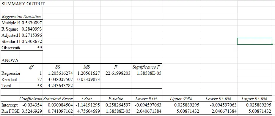
Table 4: Beta Computation of Tullow Oil Plc

The above table shows the results of the conducted regression analysis related to the dependent variable (company stocks return) and independent variable (Market returns) for Tullow Oil Plc. In beta value of the company mostly represents the level of market volatility integrated with the 5 years stock price of the company (in.investing.com, 2025). The beta value was 2.20 which is grated that the suitable range of 1 indicates high volatility in the stock price. The respected intersect value and the covariance value of the two variables are also very high indicating huge variation in the share prices.

The R-square value and the adjusted R-square value of the conducted regression analysis were 0.284 and 0.271. Both of the values are less than the ideal value of 0.5 indicating a low correlation between the variables. The P value of the regression analysis was less than the ideal value of 0.05 and the coefficient value was 3.524. The positive coefficient value indicates that they are proportional to each other. The changes in the stock price return of TWL positively affect the overall market price changes.

SHEL Plc

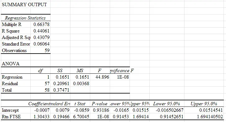
Table 5: Beta Computation of Shell Plc

The above regression analysis shows the relation between the stock price of the market (FTSE 100) and the stock price of SHEL Plc. The R-value of the above regression result was 0.93186 which was significantly lower than the ideal value range of 0.5 to 0.7. The low R-square value suggests that the independent variable which is the company share price was not effective in explaining the changes in market prices (in.investing.com, 2025). The P value of the regression analysis was also lower than the ideal value of 0.05 the significance of the regression analysis. For analyzing the mistake risk or beta of SHEL Plc slope and covariance values were evaluated. The slope value was 83.85278382 which indicates that there is slight volatility in the stocks of SHEL Plc, however, it was very low and considerable. The covariance value was also significantly low showing less variating the stock prices of SHEL Plc compared to Market prices fluctuation.

Harbour Energy Plc.

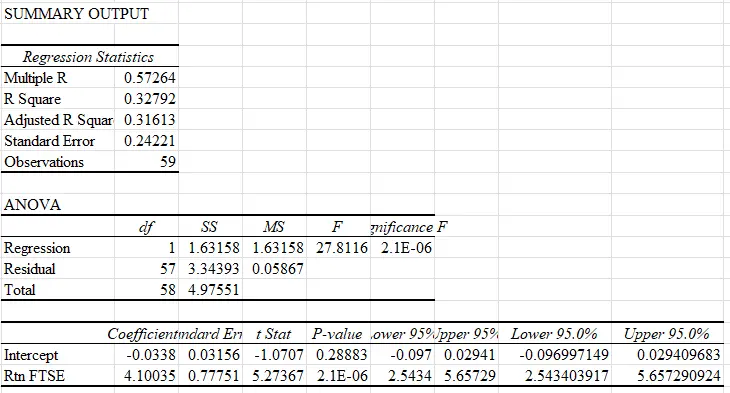
Table 6: Beta Computation of Harbour Energy Plc

The above tables show the beta values and the regression result of Harbour Energy Plc. The company has a beat value of 0.07 which is much less than the limited value of 1. This indicates that the volatility present in the stock price of Harbour Energy Plc. was very low. The results of the conducted regression analysis related to market returns and returns of Harbour Energy Plc. were the R-square and the adjusted R-square values of 0.32 and 0.31. This indicates a low correlation between the two variables (in.investing.com, 2025). The two variables have a coefficient value of 4.1 which is comparatively high and positive. The positive coefficient value indicates a positive and non-linear relation between the variables. The changes in the stock price returns of Harbour Energy Plc. significantly impacts the market stock price change.

BP Plc.

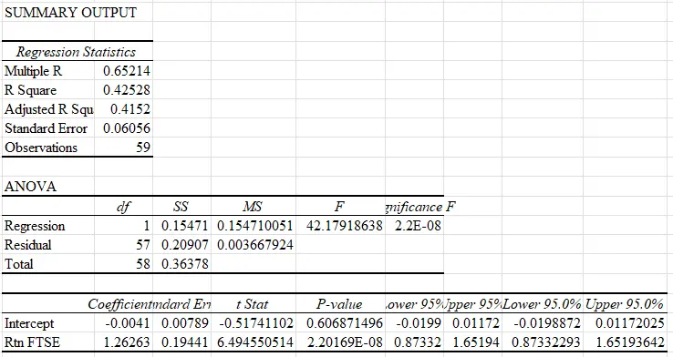
Table 7: Beta Computation of BP Plc

The above table mostly represents the beta computation of BP plc as per the above table it was easy to understand The R-value of the above regression result was 0.6068 which was significantly lower than the ideal value range of 0.5 to 0.7. The low R-square value suggests that the independent variable which is the company share price was not effective in explaining the changes in market prices. The P value of the regression analysis was also lower than the ideal value of 0.05 the significance of the regression analysis (in.investing.com, 2025). For analyzing the mistake risk or beta of BP Plc slope and covariance values were evaluated. The slope value was 4.24759067 which indicates that there is slight volatility in the stocks of BP Plc, however, it was very low and considerable. The covariance value was also significantly low showing less variating the stock prices of BP Plc compared to Market prices fluctuation.

Conclusion

The conducted financial analysis with the help of stocks and financial data of the four companies includes the time services analysis, descriptive analysis, autocorrelation analysis, and performance comparison. The conducted regression analysis concludes that the profitability ratio of all the companies is collected with only the employee ratios. The time series analysis also highlights that only the most current share prices of the company were related newest historical share prices. The companies have volatility in their share price value because of high fluctuations. With that in mind, the investors are recommended to invest in these companies or the sectors with their own risk tolerance. Because as the risk increases there is also a high chance of profitability.

References

• Chen, W. H., Uribe, M. C., Kwon, E. E., Lin, K. Y. A., Park, Y. K., Ding, L., & Saw, L. H. (2022). A comprehensive review of thermoelectric generation optimization by statistical approach: Taguchi method, analysis of variance (ANOVA), and response surface methodology (RSM). Renewable and Sustainable Energy Reviews, 169, 112917. Retrieved on; 10.02.2025
• Diggle, P., & Giorgi, E. (2024). Time series: a biostatistical introduction. Oxford University Press.
• Haddad, V., Huebner, P., & Loualiche, E. (2021). How competitive is the stock market? theory, evidence from portfolios, and implications for the rise of passive investing. Theory, Evidence from Portfolios, and Implications for the Rise of Passive Investing (April 7, 2021)
• Lucky, A. L., & Elfreda, E. N. (2024). Cost of governance and deficit financing in Nigeria: An application of Auto Regression Distributive Lag (ARDL) Model. International Journal of Economics and Financial Management (IJEFM), 9(2), 1-20.
• Sullivan, J. H., Warkentin, M., & Wallace, L. (2021). So many ways for assessing outliers: What really works and does it matter?. Journal of Business Research, 132, 530-543.
• Tsushima, E. (2022). Interpreting results from statistical hypothesis testing: understanding the appropriate P-value. Physical therapy research, 25(2), 49-55.
• Yu, Z., Guindani, M., Grieco, S. F., Chen, L., Holmes, T. C., & Xu, X. (2022). Beyond t test and ANOVA: applications of mixed-effects models for more rigorous statistical analysis in neuroscience research. Neuron, 110(1), 21-35.
• Yuan, D., Gazi, M. A. I., Harymawan, I., Dhar, B. K., & Hossain, A. I. (2022). Profitability determining factors of banking sector: Panel data analysis of commercial banks in South Asian countries. Frontiers in psychology, 13, 1000412.