MN5615 Quality Management and Reliability Assignment Sample

• Type Assignment
• Downloads543
• Pages8
• Words1935

Part A: Quality Management

Q1. (a)

Seven basic Quality Tools are useful in the identification of the quality problems in processes. Some of the basic tools of quality control are the 'fishbone diagram' used to determine the causes of a particular effect, the 'check sheet', which is used in the collection of data, the 'control chart' used in testing the stability of a process, the 'histograms' used in the display of data, the 'Pareto chart', which is used in ranking problems, concepts often explained in assignment help in UK and the 'scatter diagram' used in testing relationships between factors. The seven new quality tools include Hoshin Plan, Affinity Diagram, Tree Diagram, Interrelationship Digraphs, Matrix Diagrams, Matrix Data Analysis, Arrow Diagram, and PDPC (Hamel, and Tan, 2022). Thus, the basic tools are effective in such operational problems, at the same time the new tools are more suitable for solving complex issues, dealing with team involvement, and implementing the long-term strategy for Quality Management.

Q1. (b)

The seven basic quality tools deal with the principle that it is better to address simple quality problems. They are mainly applied in data analysis, process control and problem solving by utilizing for example control chart for stability and a Pareto chart for problem revisiting. On the other hand, the seven new quality tools introduced here are used for more sophisticated problem-solving, control planning and decision-making. They focus more on a proactive mindset and pro-actively managed; for example, using affinity tools in order to cluster ideas or matrix tools to examine relationships (Pargaonkar, 2021). Thus, the basic tools are effective in such operational problems, at the same time the new tools are more suitable for solving complex issues, dealing with team involvement, and implementing the long-term strategy for quality management.

Q2.

As per the provided data, the specific value of the limit is 25.0±0.1 mm. This means the upper limit value, USL = 25.1 mm, and the lower one value, LSL = 24.9 mm. For the determination of the capability indices, the mean of the overall values, and the std. dev. of the overall values are needed. This defines the formula as, the minimum value of ((USL-mean)/(3*std. dev.), (mean-LSL)/(3*std. dev.)). As per the calculation, the mean value of all overall is 25.06, and the std. dev. value of those data is 0.022. So, the value of capability indices = min((25.1-25.06)/(3*0.022), (25.06-24.9)/(3*0.022)) = min(0.606, 2.424) = 0.606.

The Cpk value computed was 0.606 thus implying that the process is not capable of delivering pipes to the desired tolerance of 25.0 ± 0.1 mm. A calculated Cpk below 1.0 reveals that the spread of the process is too large in relation to the specification limits around which the measurement should ideally be distributed. This low coefficient of variation indicates that the process is not symmetrical; this is evidenced by the position of the mean closer to the upper limit (25.06 mm than the 25.1 mm). To enhance the capability, improvements that shift the centre line in the process mean towards the target and decrease process variability is required prior to the implementation of the process at full scale.

Q3.

The idea behind SPC is sampling and controlling a process in order to improve efficiency and make it consistently conform to predetermined expectations. SPC enables one to distinguish between normal variation and assignable variation hence preventing special causes from occurring. When it comes to controlling the outside diameter of pipes an X-bar and R chart is appropriate. The X-bar chart observes the average diameter shift over time while the R chart observes the range of variation in each sample. What's more, plotting the sample means and ranges enables the identification of shifts or trends in the process (Carey et al., 2022). With these control charts, you can judge the process control status, such as outside control limits, or have rising or declining trends, so that timely measures can be taken to adjust the equipment or training of operators to maintain process quality and stabilize at specified standards.

Q4. (a)

The evaluation of the overall savings of the investment is determined by using the function of Taguchi loss. This highlights, Lav = k⋅MSD≈k[s^2 +(y−m)^2]. In this case, Lav => average of Taguchi loss, y => nominal target, k => constant, m => mean value, and s^2 => variance. For this case, let k => 1. So, the mean values of the data = (50+45+46+54+48+47 )/6 = 48.33 lb.

So, the variance value s^2 is,

((50-48.33)^2+(45-48.33)^2+(46-48.33)^2+(54-48.33)^2+(48-48.33)^2+(47-48.33)^2)/(6-1) = (2.79+11.09+5.42+32.15+0.11+1.77)/5 = 10.67. So, the value of MSD => s^2+(y-m)^2 = 10.67 + (45 - 48.33)^2 = 10.67 + 11.09 = 21.76.

Now for the new assembly, these values are evaluated as,

Mean => 44.58, and the value of variance => 1.04. So, the value of MSD for new assembly => 1.04 + (45-44.58)^2 = 1.04+0.18 = 1.22. So, the Lav for the original data is k*MSD = 1*21.76 = 21.76 lb^2, and the Lav for the new one is k*MSD = 1*1.22 = 1.22 lb^2. So, the saving is 21.76-1.22 = 20.54 lb^2.

This describes the saving as around £20.54 /unit which highlights that the new assembly has a good saving value.

Q4. (b)

A t-test is a statistical method that allows a researcher to compare the mean of two groups in order to judge whether the difference between the mean is statistically significant. Using the given t-table locate the t value for a two-tailed test by taking degrees of freedom (df=n1+n2−2df = n_1 + n_2 - 2df=n1+n2−2äter α=0.05\alpha = 0.05α=0.05. Subtract the Titled t-value from the critical value from the table of a given coefficient. If the absolute t-value tops the found critical value, we reject the null hypothesis and corroborate a difference in the quality of the two assembly operations.

Part B – Reliability

Q5.

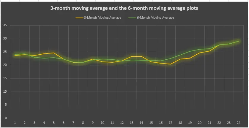
Figure 1: Moving average value plots of 3 and 6-month

This case shows how failures observed for 24 months have been plotted by using 3-month and 6-month mobile averages. The 3-month moving average is much more sensitive to the changes in data and that is why it is represented by the yellow colour line. On the other hand, the 6-month moving average (green line) significantly smooths the fluctuations and exhibits a more widespread direction. These averages show that over time, failure numbers rise especially when viewed towards the later months. The 3-month average is slightly higher than the 6-month average, mainly attributed to all the above because the calculation of 6 months takes a longer timeline. Such trends call for examining possible causes for the failure increase, especially in the last months of the given year. This case shows how failures observed for 24 months have been plotted by using 3-month and 6-month moving averages, which is an essential technique in Reliability to monitor and improve system performance over time."

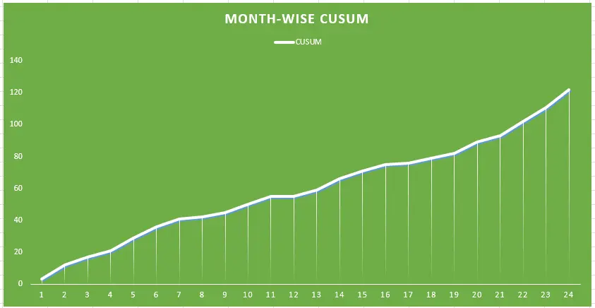
Figure 2: Month-wise CUSUM

This CUSUM plot indicates the accumulation of the deviation of monthly failures from the target of 18 within 24 consecutive months. It is demonstrated by the flow of the curve that every month, the number of failures is above the designated goal. After the first few months, the curves show a linear increase but from the mid-period, there is much more inclination showing deviation. Such continuous rise indicates potential process wastes or some rising concerns that require attention. The plot is an equally important tool for monitoring trends for the variances column to determine the tendencies and call out the need for taking corrective actions for failures that are near the target.

Q6. 1)

As per the data given for the failure time of the various 8 products which are 35, 48, 31, 39, 59, 53, 75, and 66 days. So, the calculated, MTTF is evaluated as the sum of failure time divided by total no. failure. So, MTTF = (35+48+31+39+59+53+75+66)/8 = 50.75 days.

Q6. 2)

The product reliability is estimated by using, the formula 'exponential distribution', which is expressed as, e^(-λT). Here λ => rate of failure, T => time which is 60 days in this case. The value of λ is evaluated as 1/MTTF = 1/50.75 = 0.0197. So, the value of reliability = e^(-0.0197*60) = 0.3067 which is 30.67%.

Q6. 3)

Comparison with a fixed testing rate as implied by exponential distribution might be appropriate if the product is in its early phase and characterised by random failures arising from basic design and manufacturing flaws or environmental influences. Again, the failure times were all over from 31 to 75 and some of the products failed at 90 still in operation, this is an indication that the failure was likely to be more or less the same. Nevertheless, in case when the product deteriorates with time, the rate of failure may also grow, which means that the assumption about constant failure rate does not seem valid in this case (Iafrati et al., 2024). Moreover, there could be added statistical measures to get a clearer picture.

Q7.

The overall reliability of the given block diagram is resolved by using some necessary evaluation steps. In the first evaluation point, the reliability of the top series is evaluated. Here top two series values are 0.75 and 0.95. As those two are in a series, the value of reliability for these is (0.95*0.75) = 0.7125. Now the reliability of the bottom series is evaluated as (0.75*0.8) = 0.6. Now the series is combined with the parallel one whose value is 0.85. So, for this, the reliability is (1 - [(1-0.7125)*(1-0.85)*(1-0.6)]) = (1-(0.2875*0.15*0.4)) = 0.98. Now this value is in series with the first value which is 0.95. So, the overall reliability is, (0.95*0.98) = 0.931.

Q8. a)

As per the provided tabular data, 6, 9, and 10 units did not fail at the end of the testing process. So, the values of 6, 9, and 10 are removed and the sorted failed data are as below,

Failure time (hr)	Median Rank (MR)
600	0.095
820	0.229
980	0.365
1150	0.5
1300	0.635
1500	0.770
1800	0.905

Table 1: Failure-wise Ranking

The sorted data describes the failure in ascending order and as per this ranking is assigned.

Now the median rank is evaluated as, (i-0.3)/(n+0.4), where n => total number of failures = 7, and i => the instance values such as 1, 2, 3, and so on.

i) i => 1,

Median rank = (1-0.3)/(7+0.4) = 0.095.

ii) i => 2,

Median rank = (2-0.3)/(7+0.4) = 0.229.

iii) i => 3,

Median rank = (3-0.3)/(7+0.4) = 0.365.

iv) i => 4,

Median rank = (4-0.3)/(7+0.4) = 0.5.

v) i => 5,

Median rank = (5-0.3)/(7+0.4) = 0.635.

vi) i => 6,

Median rank = (6-0.3)/(7+0.4) = 0.770.

vii) i => 7,

Median rank = (7-0.3)/(7+0.4) = 0.905.

Failure time (hr)	Median Rank (MR)
600	0.095
820	0.229
980	0.365
1150	0.5
1300	0.635
1500	0.770
1800	0.905

Table 2: Failure-wise Median Rank

Q8. b)

Failure time (hr)	Median Rank (MR)	Cumulative Percent Failure (CPF) (%)
600	0.095	9.5
820	0.229	22.9
980	0.365	36.5
1150	0.5	50
1300	0.635	63.5
1500	0.770	77
1800	0.905	90.5

Table 3: Failure-wise Cumulative Percent Failure (%)

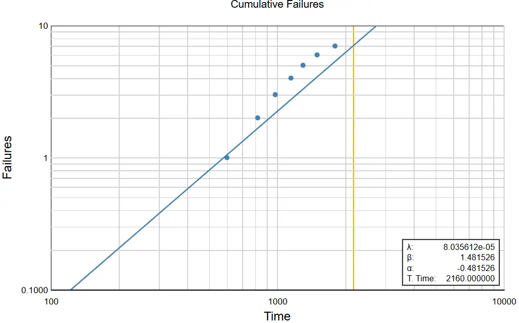
Figure 3: Cumulative failure with failure time

Q8. c)

Failure time (hr)	Cumulative Percent Failure (CPF)	X = ln(t)	Y=ln(ln(1/(1−F(t))))
600	0.095	6.396	2.417
820	0.229	6.706	3.036
980	0.365	6.888	3.443
1150	0.5	7.050	3.665
1300	0.635	7.170	3.811
1500	0.770	7.313	3.984
1800	0.905	7.495	4.109

Table 4: X, and Y evaluation

MN5615 Quality Management and Reliability Assignment Sample

Liked This Sample? Hire Me Now

Karen Evans 9 Years | PhD

Evaluation of Y is determined as bX+C. The b is evaluated as the sum of X, and the sum of Y. It also includes the sum of X^2, and also the sum of (X*Y). So, the value of b which is the shape factor (b), this value is (n*(sum(x*y)-(sum(X)*sum(Y)))/(n*sum(X^2)-(sum(X))^2). On the other hand, the intercept value (c) is evaluated as (sum(Y)-b(sum(X)))/n. Here the value of n => 7. The characteristic time for this is evaluated as, e^(-c/b). So, the value of b = 1.56, and the value of failure characteristic time is 117.72 hr.

Since b>1 this shows that it fails under a wear-out failure mode Different a and b emerge from the data when the above shadings are done, it can be explained by the fact that the particular unit in regard to peculiarities and type of utilisation is different. The fact that Control Objectives degrade or wear out with time implies that failures are more likely to happen at later times.

Q8. d)

The reliability of the data for 900 hr is evaluated as (1-e(-(900/117.72)^1.56)) = 3.49*10^-11. On the other hand, the failure probability from 900 to 1000 is evaluated as 3.4*10-11.

References

• Carey, C.C., Woelmer, W.M., Lofton, M.E., Figueiredo, R.J., Bookout, B.J., Corrigan, R.S., Daneshmand, V., Hounshell, A.G., Howard, D.W., Lewis, A.S. and McClure, R.P., 2022. Advancing lake and reservoir water quality management with near-term, iterative ecological forecasting. Inland Waters, 12(1), pp.107-120.
• Hamel, P. and Tan, L., 2022. Blue–green infrastructure for flood and water quality management in Southeast Asia: evidence and knowledge gaps. Environmental Management, 69(4), pp.699-718.
• Iafrati, A.C., Cappadozzi, G., Silvestri, C. and Pinto, M., 2024. An Italian InterLaboratory comparison on personal dose equivalent for dosimetry services: promoting measurements reliability and addressing new digital challenges. The European Physical Journal Plus, 139(3), p.269.
• Pargaonkar, S., 2021. The Crucial Role of Inspection in Software Quality Assurance. Journal of Science & Technology, 2(1), pp.70-77.